Storing geodata in neural networks

Chapter 6 · Spherical harmonics

Deutsche Fassung · Translated from the German original.

Chester with his blue cap uses tweezers to set mosaic pieces into a globe made of many blue, green and ochre tiles. On the left stands Aiko, a glowing neural network, in front of a sorting box; more mosaic pieces lie on the table.

Contents:

Which fixed, ordered set of patterns fits the sphere exactly
How the Earth can be assembled from these spherical harmonics
Why they become expensive for fine detail

This chapter extends chapter 5. You can also skip it.

Starting point

In chapter 5, 128 stripe patterns with random direction and random spacing were laid over the Earth. That works well, but it is a makeshift: straight stripes do not fit a sphere exactly.

Mathematicians have long known an ordered set of such patterns that is made precisely for the sphere. They are called spherical harmonics. They are the counterpart on the sphere of the Fourier analysis from chapter 5.

Spherical harmonics

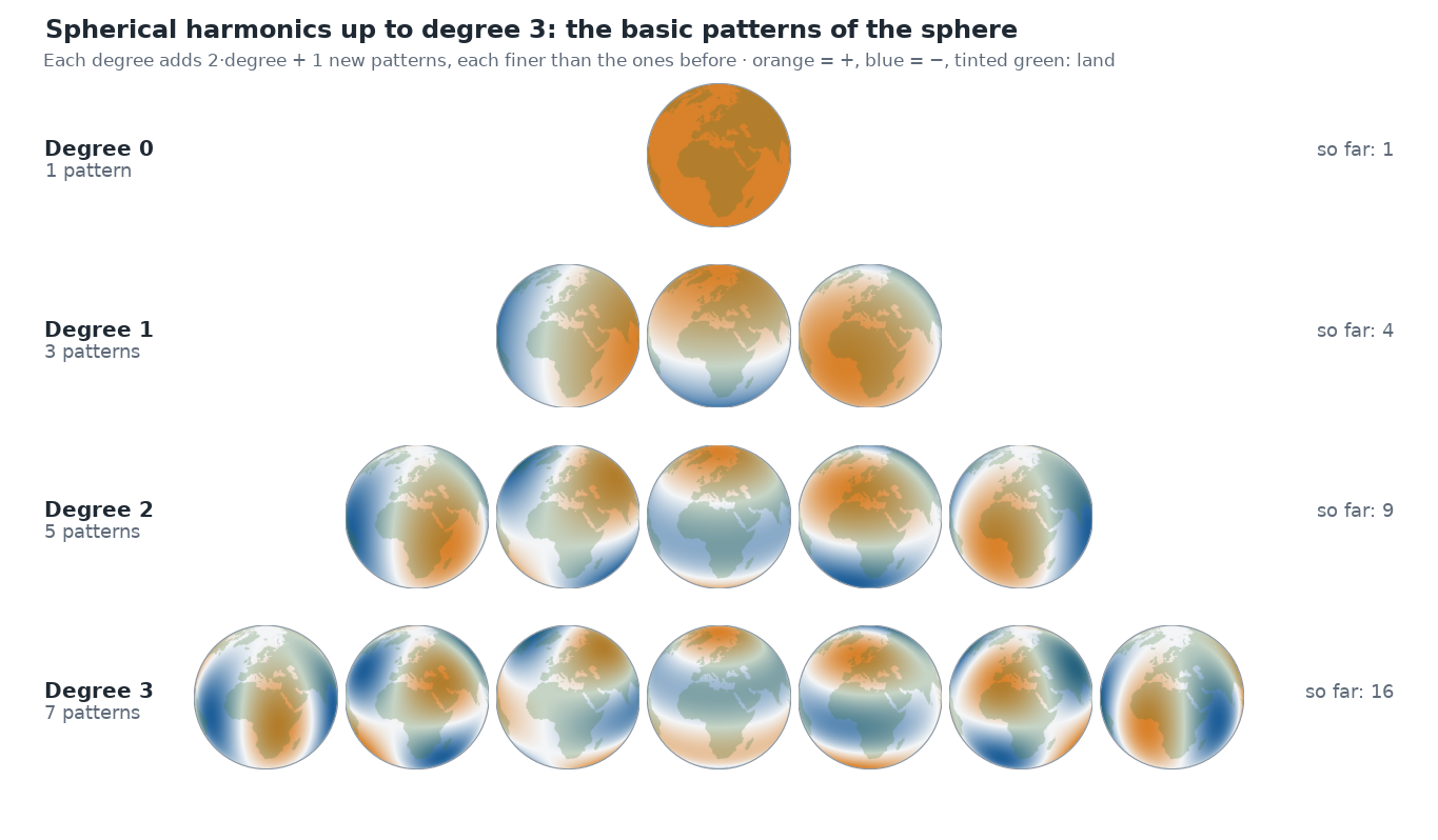
The spherical harmonics are ordered by their degree. Each degree brings different patterns, each finer than the ones before:

Spherical harmonics of degrees 0 to 3 on globes, arranged as a pyramid. Degree 0: a single pattern, the whole sphere the same. Degree 1: three patterns, each with one half positive and one negative. Degree 2: five patterns with four fields or bands. Degree 3: seven even finer patterns. Up to degree 3 there are 16 patterns in total.

As with the stripe patterns in chapter 5, you get a wave here too if you walk across the sphere and plot the values:

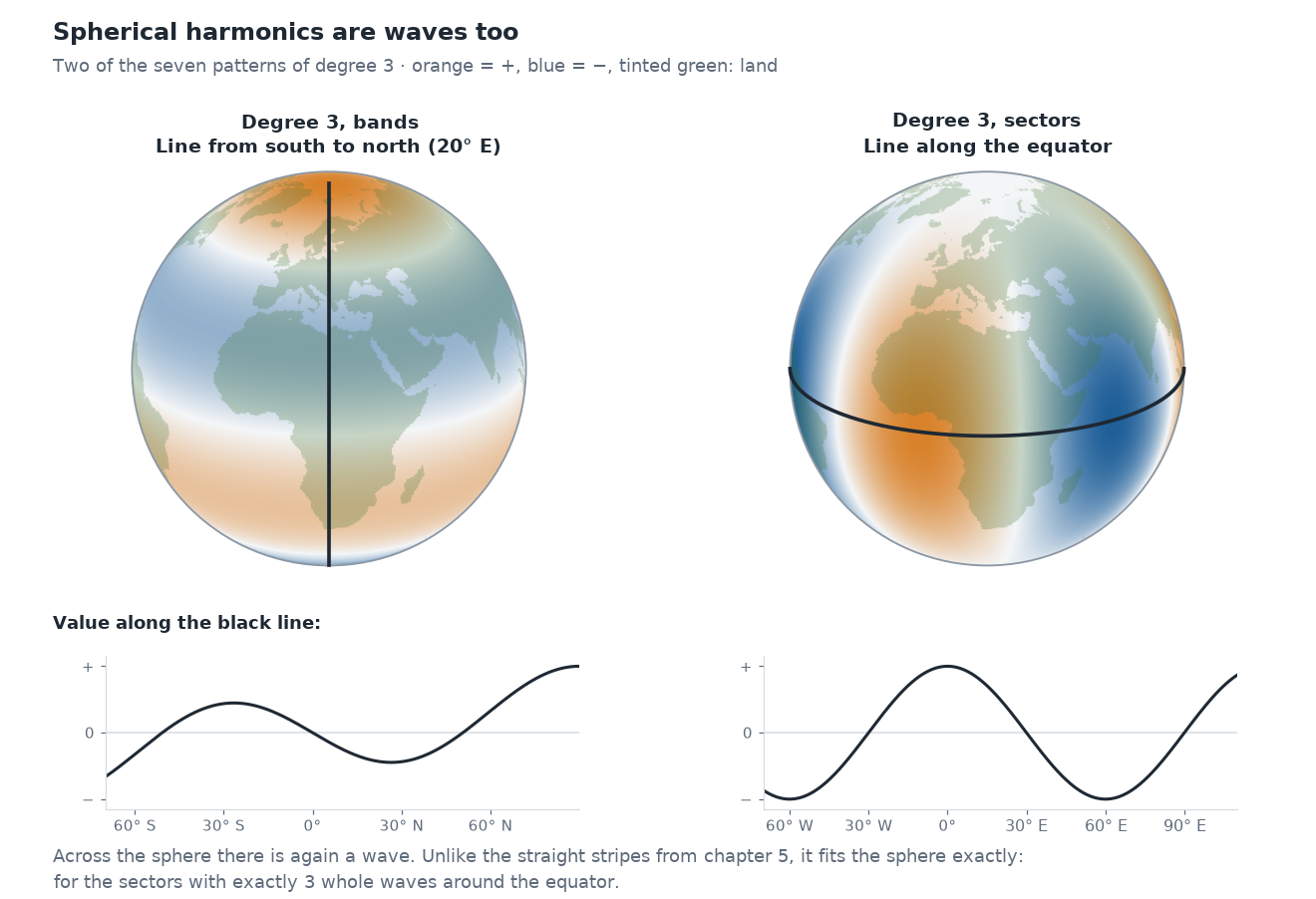
Two spherical harmonics of degree 3 on globes. On the left a pattern of bands with a line from south to north; below it the values along the line: a wave that rises to its maximum towards the North Pole. On the right a pattern of sectors with a line along the equator; below it an even wave with a peak at 0° and troughs at 60° west and 60° east – exactly three waves around the Earth.

Unlike the straight stripes from chapter 5, these waves fit the sphere exactly: along the equator, the sector pattern has a whole number of waves – exactly three for degree 3.

Degree 0: a single pattern, the same everywhere. It stands for the mean elevation.
Degree 1: three patterns. Each divides the sphere into a positive and a negative half – one into north and south, two into east and west.
Degree 2: five patterns; the sphere is divided into four fields or into bands.
Each further degree brings 2 · degree + 1 new patterns, and the fields become smaller.

Up to a degree L there are therefore (L + 1)² patterns. The finest wave is roughly 40 000 km divided by L long – the Earth's circumference divided by the degree:

highest degree L	patterns in total	shortest wave
2	9	about 20 000 km
8	81	about 5 000 km
16	289	about 2 500 km
40	1 681	about 1 000 km
100	10 201	about 400 km

Unlike the random stripes from chapter 5, these patterns are complete: up to their degree no wave is missing, and none appears twice. And they are orthogonal – each pattern describes something that no other pattern describes. That is why geodesy has used them for decades to describe the shape and the gravity field of the Earth. The Earth gravity model EGM2008, for example, consists of the weights of spherical harmonics up to degree 2190 [1].

The Earth from spherical harmonics

With these patterns you can assemble the Earth – just like the Alpine profile from waves in chapter 5. Each pattern gets a weight, and all of them are added up. The higher the degree, the more patterns are available and the sharper the Earth becomes:

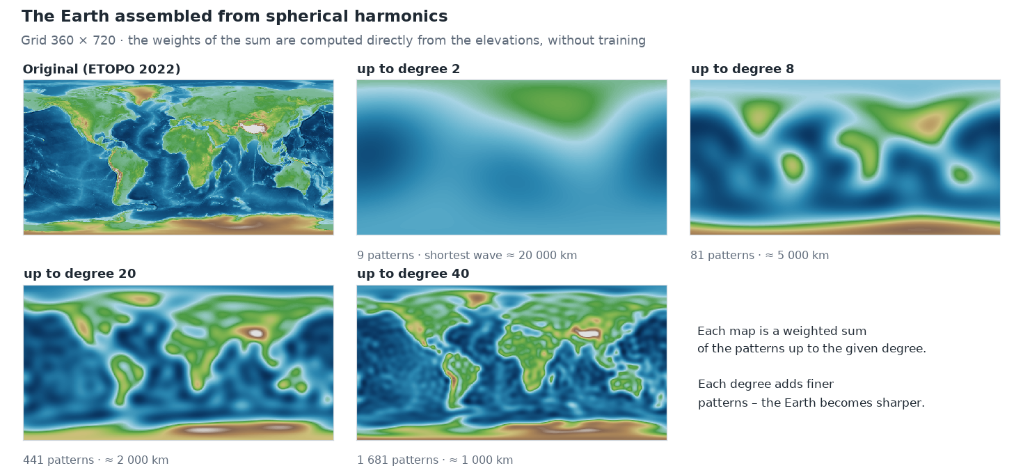
Five world maps: the original and the Earth assembled from spherical harmonics up to degree 2, 8, 20 and 40. Up to degree 2 only a rough difference between the northern hemisphere and the Pacific is visible, up to degree 8 continents appear as blobs, up to degree 20 their outlines are recognisable, up to degree 40 also peninsulas, mountain ranges and Antarctica.

This is the simplest model from chapter 3, only with different inputs: a weighted sum, without hidden layers and without kinks. Each pattern is an input, each weight belongs to one pattern.

With spherical harmonics the right weights can even be computed directly, without training – that is how the figure above was made. If you instead train a network without hidden layers on these inputs, training finds the same weights. Such a network is thus exactly the classical representation used in geodesy.

Spherical harmonics as input for a network

Instead of the random stripes from chapter 5, the spherical harmonics can also be used as input for a network with hidden layers. For a place you look up – as in chapter 5 – the value of each pattern at that point. Up to degree 16 these are 289 numbers instead of 256.

The network can then combine the patterns further with its kinks and so also form shapes that are finer than the shortest wave of the input.

The app offers two presets for this:

Preset	Degree L	Inputs	Hidden layers	Weights	Size	Compression ratio
Spherical harmonic expansion (L = 40, linear)	40	1 681	0	1 682	6.6 KB	693
Spherical harmonics (L = 16)	16	289	4	86 785	339 KB	13
for comparison: Fourier MLP (recommended), chapter 5	–	256	4	82 561	323 KB	14

The linear variant is tiny: it needs only one weight per pattern and is around 700 times smaller than the grid. In return it shows no detail below about 1 000 km.

The price of completeness

As elegant as spherical harmonics are – for fine detail they become expensive. Because they are complete, every finer wave needs all directions at once: for waves 400 km long you need more than 10 000 patterns, for 100 km already more than 160 000. Each pattern is an input, and each input costs one weight per neuron in the first layer of a network.

The random stripes from chapter 5 are more economical here. They do not cover every direction systematically, but they reach short waves with as few as 128 patterns. The network can then pick the right ones from many directions.

	random stripes (chapter 5)	spherical harmonics
choice of patterns	random, from a seed	fixed and ordered
fit the sphere exactly	approximately	yes
complete up to a wavelength	no	yes
number of inputs for short waves	small (e.g. 256)	grows very quickly
computing effort	low	high, especially for large L

Which variant matches the elevations better depends on the network size and the degree. For networks of the same size the two are close: with 4 000 training steps on the standard grid, Spherical harmonics (L = 16) reaches a weighted RMSE of 241 m, Fourier MLP (recommended) 245 m. The linear model up to degree 40 reaches 631 m with only 6.6 KB – more accurate than the simple network from chapter 2 with 706 m, which is 30 times as large. All values are in the appendix with the measurements.

Try it out

In the sidebar under 2 · Network, choose the preset Spherical harmonic expansion (L = 40, linear) and open Architecture details.

Positional encoding now shows spherical. The Maximum degree L slider sets the highest degree. Below it the app shows the number of patterns and the shortest wave. Hidden layers is set to 0: a linear model.

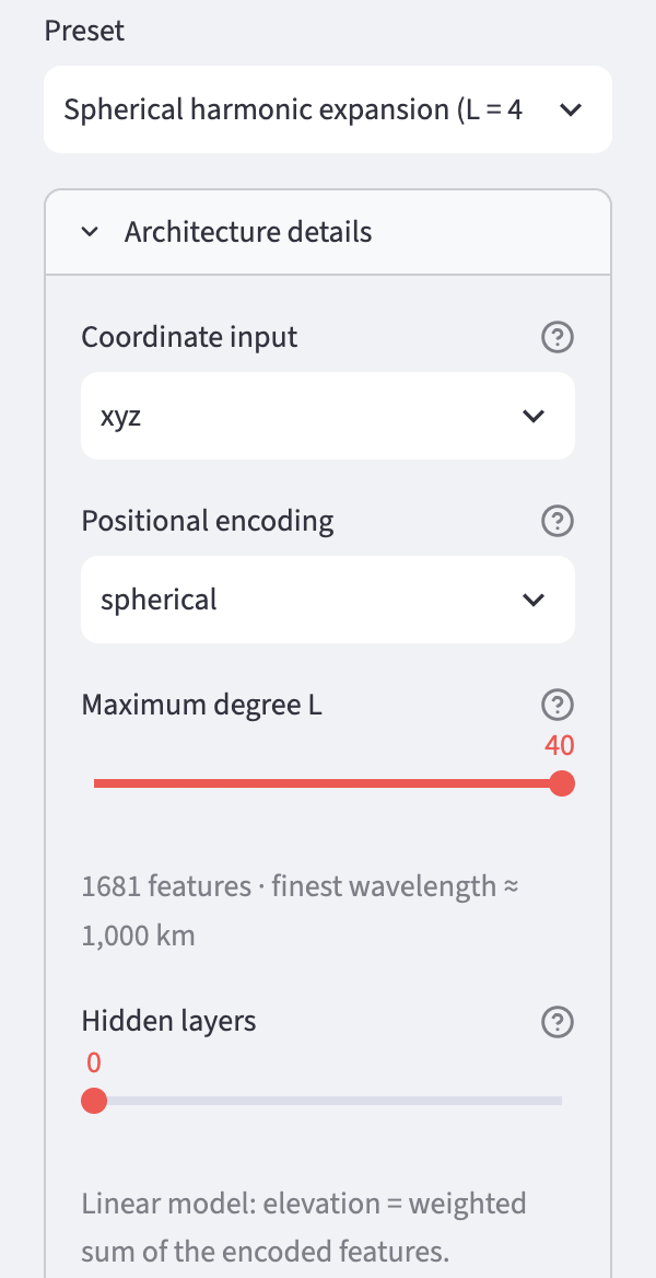
Sidebar with Architecture details expanded: preset Spherical harmonic expansion, Positional encoding spherical, Maximum degree L 40, below it 1681 features and finest wavelength about 1,000 km, Hidden layers 0 and the note Linear model.

Train and look at the result in the Maps & Error tab. It should look similar to the map "up to degree 40" above.

Then choose the preset Spherical harmonics (L = 16), train and compare the result with Fourier MLP (recommended) from chapter 5.

Note on computing time: With a large degree, training becomes slow because very many patterns have to be computed for every place. On an Apple M4, 4 000 steps take about 5 minutes with L = 40 and just under 2 minutes with L = 16; Fourier MLP (recommended) needs a little over 1 minute. For first attempts, a smaller L or a smaller Grid resolution is worthwhile.

Ideas to explore further

For the linear model, set Maximum degree L to 8, 20 and 40 and compare the maps with the figure above.
For the linear model, increase Hidden layers from 0 to 2. What happens to the number of weights – and to the detail?
For Spherical harmonics (L = 16), lower the degree to 8. How much worse does the result get, and how much smaller the file?