Storing geodata in neural networks

Chapter 7 · SIREN

Deutsche Fassung · Translated from the German original.

Chester with his blue cap and Aiko, a glowing neural network, surf at night over glowing waves on a sea; the globe rises on the horizon.

Contents:

How a neuron computes with a sine instead of a kink
Why such a network needs the right initialisation
How it does on the world map compared with the Fourier features

Instead of turning the input into waves (chapter 5), here every neuron itself computes with a sine curve. This chapter extends chapter 5. You can also skip it.

Starting point

In chapter 5 the neural network got waves as input, the Fourier features. The neurons themselves stayed as they were in chapter 3: weighted sum and kink.

In 2020, Sitzmann and colleagues proposed a different approach [1]: the input stays as it is – here the three numbers x, y, z from chapter 4 – but every neuron passes on its sum not with a kink but through a sine (as activation function). Such a network is called SIREN, short for Sinusoidal Representation Network.

Sine instead of kink

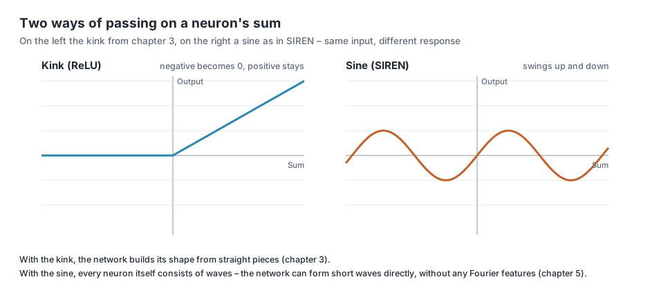
Two diagrams side by side. On the left the kink (ReLU): for negative sums the output is 0, for positive ones it rises in a straight line. On the right the sine: the output swings evenly up and down.

A neuron in a SIREN network computes in three steps. The example is Regensburg from chapter 4 with x = 0.64, y = 0.14 and z = 0.75; the weights are made up: w₁ = 0.2, w₂ = −0.5, w₃ = 0.1 and the bias b = −0.1.

1. The weighted sum – exactly as in chapter 3: each input times its weight, add everything up, add the bias.

\[ s = w_1 \cdot x + w_2 \cdot y + w_3 \cdot z + b \]

For Regensburg: s = 0.2 · 0.64 − 0.5 · 0.14 + 0.1 · 0.75 − 0.1 = 0.128 − 0.070 + 0.075 − 0.100 = 0.033.

2. Until now: the kink. An ordinary neuron passes on the sum with ReLU – negative values become 0, positive ones stay:

\[ \text{Result} = \text{ReLU}(s) = \max(0,\, s) \]

For Regensburg: ReLU(0.033) = 0.033.

3. New in the SIREN network: the sine. Instead of the kink, the sum is multiplied by a fixed factor ω₀ (omega zero) and put into a sine:

\[ \text{Result} = \sin(\omega_0 \cdot s) \]

Sitzmann and colleagues recommend ω₀ = 30, and that is also the setting in the app. For Regensburg: sin(30 · 0.033) = sin(0.99) ≈ 0.84.

The result no longer cuts anything off but swings between −1 and +1. And because ω₀ = 30 greatly enlarges the sum, it swings quickly. Even small changes of the sum are enough for a full swing:

Sum s	−0.1	−0.05	0	0.02	0.05	0.1
ReLU(s)	0	0	0	0.02	0.05	0.1
sin(30 · s)	−0.14	−1.00	0	0.56	1.00	0.14

What this does: with the kink, the network builds its shape from straight pieces. With the sine, every neuron itself consists of waves – and every further layer combines the waves of the layer before into new, finer waves. The network can therefore form short waves directly, without any Fourier features.

SIREN on the Alpine profile

How well this works is shown once more by the Alpine profile. You know the top two rows from chapter 5; below them is a SIREN network of about the same size:

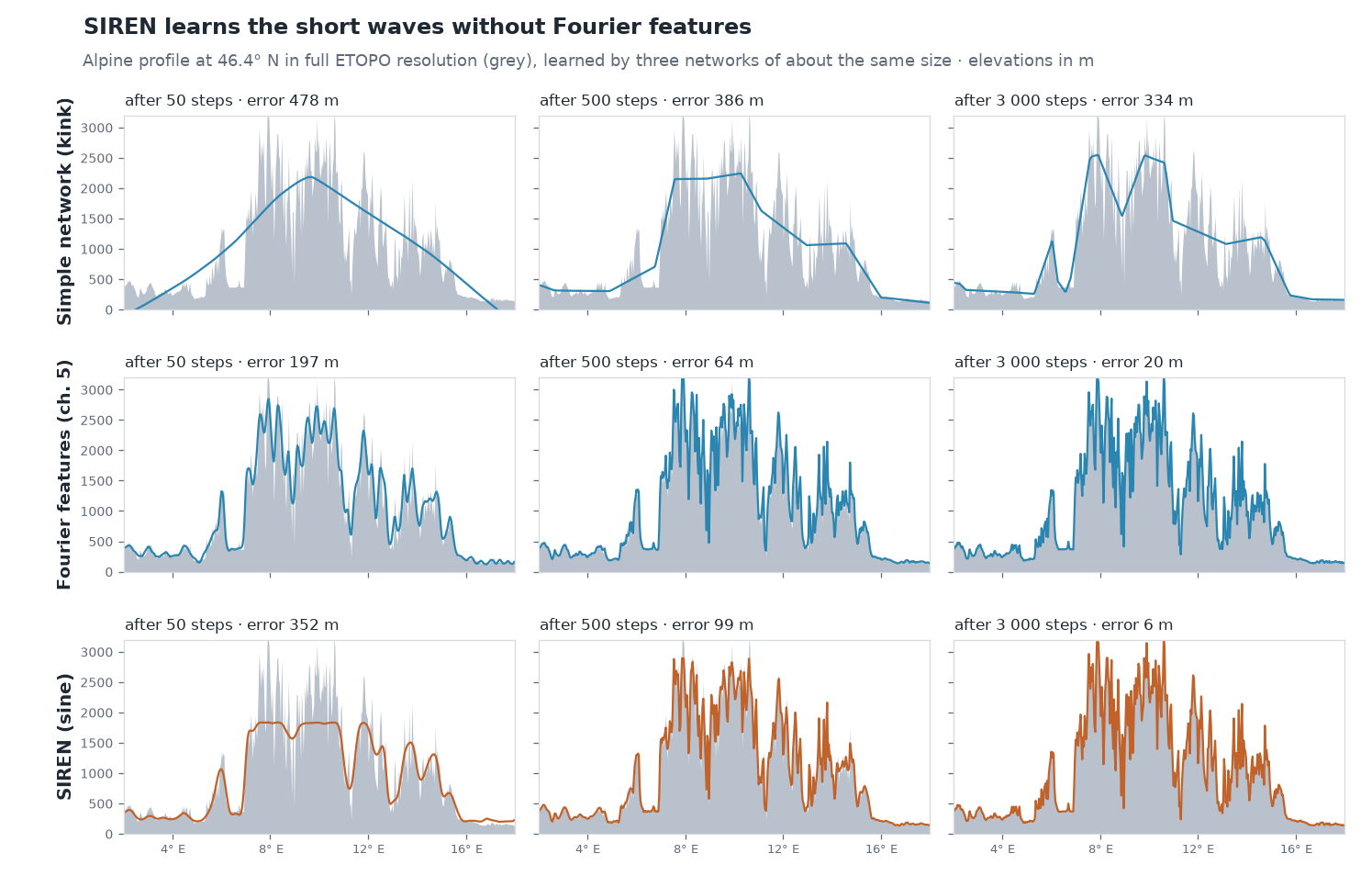
Three rows, each with three images of the Alpine profile after 50, 500 and 3 000 steps. At the top the simple network with kink: even after 3 000 steps only a rough outline, error 334 m. In the middle the network with Fourier features: 20 m after 3 000 steps. At the bottom the SIREN network: after 50 steps a rough outline with plateaus, 99 m after 500 steps, 6 m after 3 000 steps.

The SIREN network takes a little longer to get going – after 50 steps it is still rough. After that it catches up and after 3 000 steps matches the profile even more closely than the network with Fourier features.

Without the right initialisation it goes wrong

A SIREN network is sensitive to its starting weights. If they are distributed randomly as in an ordinary network, the sines swing far too fast from the start.

The network then memorises every training point perfectly – and produces noise in between.

Sitzmann and colleagues therefore prescribe a special initialisation: the weights are chosen so small that the sum before each sine varies only by about ±1 at first [1]. The network then starts with leisurely waves and builds up the fast ones only during training.

How large the difference is can be seen in an experiment: both networks learn only every second point of the Alpine profile; the points in between serve as a check.

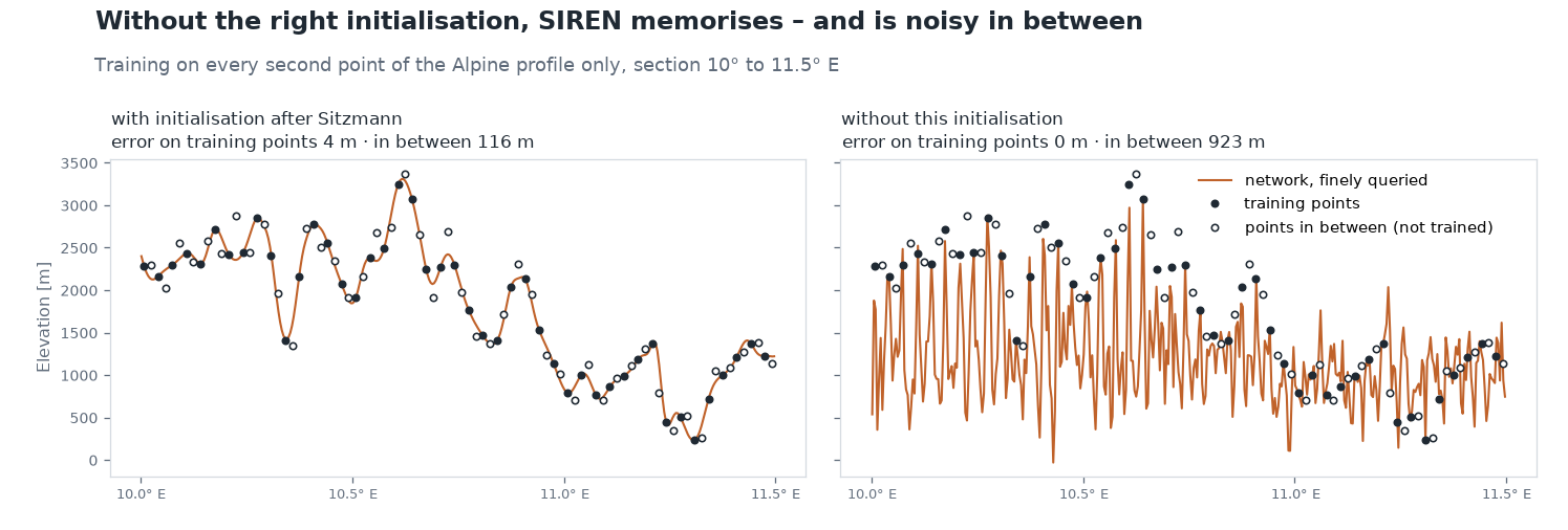
SIREN network	Error on the training points	Error on the points in between
with initialisation after Sitzmann	4 m	116 m
without	0 m	923 m

This is the same trap as a too large σ in chapter 5: waves that are too fast. For compression it is particularly treacherous, because the error curve during training looks excellent – only when querying between the grid points does the noise show. The app uses the initialisation after Sitzmann.

SIREN on the world map

On the whole Earth, again with the section of Europe from chapter 5:

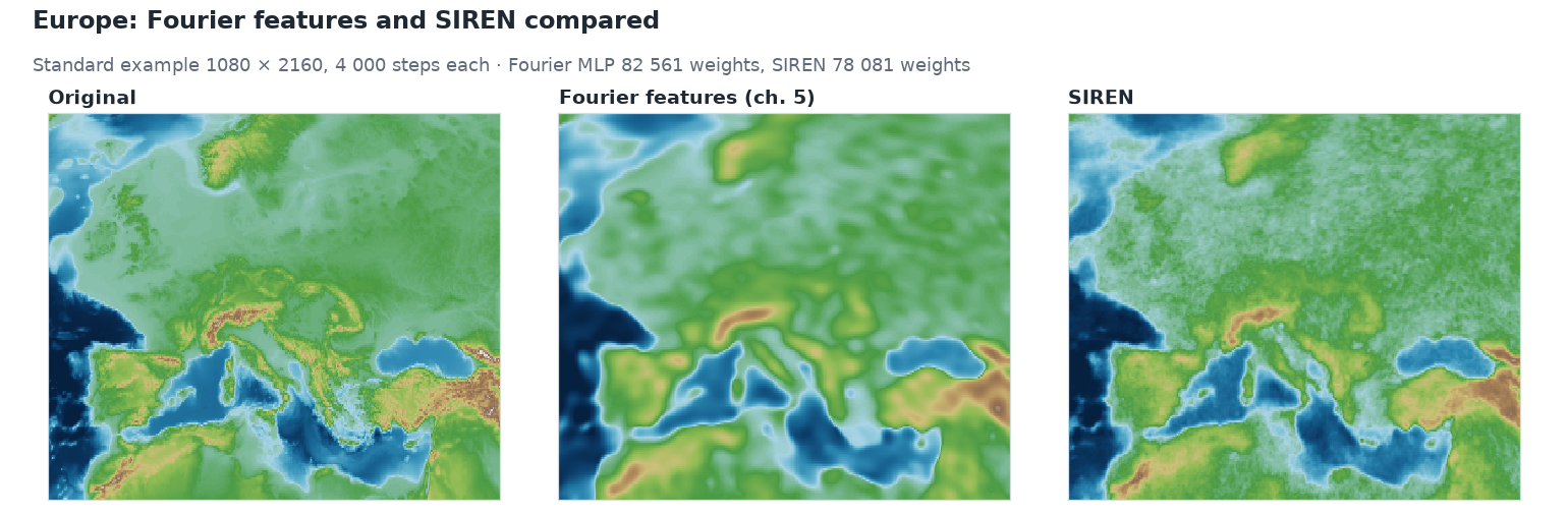
Three maps of Europe: the original, the network with Fourier features and the SIREN network. The Fourier map is soft. The SIREN map has sharper coasts and more distinct mountain ranges but shows a fine, grainy pattern on land.

The SIREN network draws coasts and mountain ranges more sharply but has a fine, grainy pattern on land – waves that have turned out a little too fast. Both networks are about the same size:

Preset	Inputs	Hidden layers	Neurons per layer	Weights	Size	Compression ratio
Fourier MLP (recommended), chapter 5	256	4	128	82 561	323 KB	14
SIREN (sine activation)	3	4	160	78 081	305 KB	15

The SIREN network has only three inputs and can therefore have more neurons per layer for the same file size. With 4 000 training steps on the standard grid, the SIREN network reaches a weighted RMSE of 233 m on average over three runs, Fourier MLP (recommended) 245 m. The SIREN network varies more, though: its three runs are 31 m apart, those of the Fourier network only 5 m. All values are in the appendix with the measurements.

What to keep in mind when saving: Because ω₀ = 30 amplifies every small change of the weights, a SIREN network reacts more sensitively to rounding than a network with kinks. This matters when saving with fewer digits – more on that in chapter 10.

Try it out

In the sidebar under 2 · Network, choose the preset SIREN (sine activation) and open Architecture details.

Positional encoding is set to none: there are no Fourier features. Activation shows siren.

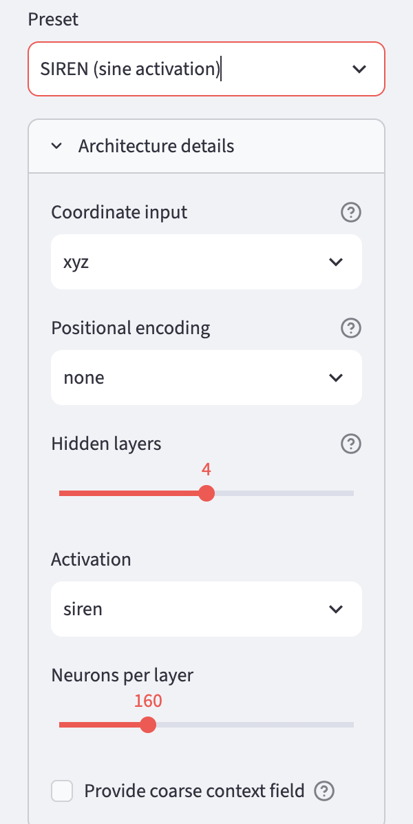
Sidebar with Architecture details expanded: preset SIREN (sine activation), Coordinate input xyz, Positional encoding none, Hidden layers 4, Activation siren, Neurons per layer 160.

Train and compare the result with Fourier MLP (recommended) in the Maps & Error tab. In the Globe 3D tab it is worth looking at mountain ranges such as the Andes or the Himalayas.

To do so, set View direction (longitude) to about −70 and Display grid to 360. You then see North and South America:

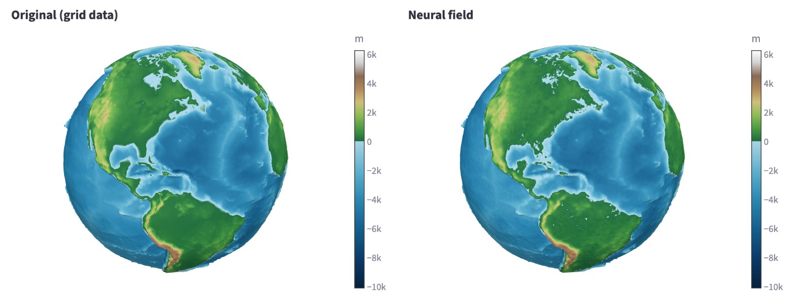
The Globe 3D tab after training the SIREN preset: on the left the original, on the right the neural field, both looking at North and South America. The Andes and the Rocky Mountains are clearly visible on both globes. On the right the land is patchier: in the Amazon basin there are small blue speckles where the network computes elevations just below zero.

The Andes come out sharply in the SIREN network. On flat land, however, the grainy pattern shows: small blue speckles, for example in the Amazon basin, which is green everywhere in the original. There the network computes elevations just below zero, and the colour scale switches to blue.

Ideas to explore further

For the SIREN preset, lower the Learning rate to 0.0003. Does the grainy pattern become weaker?
Lower Neurons per layer from 160 to 64. How much file size does that save, and how much worse does the map get?
Under Activation, choose siren once for the preset Fourier MLP (recommended). What happens when you combine Fourier features and sine?