Storing geodata in neural networks

Chapter 11 · Context and outlook

Deutsche Fassung · Translated from the German original.

Evening sun over a wide valley. On a thick branch stands Aiko, a glowing neural network, spreading its arms; next to it sits Chester with his blue cap, pointing into the distance with his paw. In the valley many small points of light glow, glowing paths wind between trees, and fields are separated from each other by borders.

Contents:

How good the results of this tutorial are compared with research
What could still be improved for grid data
Outlook: how can vector data – points, lines and areas – be represented with neural networks?

Starting point

For ten chapters it was all about a single grid: the elevations of the Earth. The standard example stores 2 332 800 elevation values in 82 561 weights, 14 times smaller than the grid, and even 28 times with float16 (chapter 10). In return it is off by around 245 m on average; with the context field it is around 186 m (chapter 8 and appendix).

This last chapter puts that into context and looks beyond the grid. Because many geodata are not grids at all, but points, lines and areas.

Context: why Huang and Hoefler compress much more strongly

The model for this series, Huang and Hoefler, reports compression ratios from 300 to over 3 000 [1]. That is 10 to 100 times what was achieved here. Is that due to poor networks?

Largely not. It is due to the data:

Smooth fields. Huang and Hoefler compress weather and climate data. Such fields mostly change evenly over large distances. In the language of chapter 5: they consist mainly of long waves. The Earth's terrain, by contrast, is rugged. Mountain ranges, coasts and deep-sea trenches are short waves, and each of them costs weights.
More dimensions. Their data are multidimensional, i.e. not only spread over the surface. A network that learns a function of many coordinates can exploit similarities between neighbouring points in time or altitude levels. A single elevation grid has nothing of the kind: every detail must come from the weights themselves.
Larger amounts of data. The larger the original, the easier a high rate becomes, as long as the network does not have to grow to the same extent. The standard grid has a good 2 million values; weather and climate data often have many billions.

For a single, rugged grid without a further dimension, rates in the range of 10 to 100 are therefore a realistic result. That is exactly what makes the example instructive: the trade-off between file size and error is clearly visible and not hidden behind an impressive number.

What could still be improved for grids

Three directions that are pursued in research and go beyond this tutorial:

Hash grids. Müller and colleagues add tables of learnable numbers at several resolution levels to a small network [2]. For a place, the matching entries are looked up and given to the network as input – a further development of the idea of the context field from chapter 8. This makes do with a much smaller network, and training is considerably faster. For compression, however, the same applies as for the context field: the tables belong to the file and must be counted honestly.

Quantisation already during training. Chapter 10 showed that float16 costs almost nothing for the Fourier MLP. With 8 bits or fewer per weight, the file would become half as large again or smaller. For this to work, the network computes with the coarser numbers already during training and learns to cope with them.

Time series. Instead of f(lon, lat), the network learns f(lon, lat, t), for example the temperature over a whole year. Time is simply another input. It is with such multidimensional data that Huang and Hoefler reach their high rates.

Outlook: vector data

A grid is a table of values at fixed grid points. Vector data are something else: individual objects with precise geometry.

Points: measuring stations, sites where animal species were found, addresses. Each point has a coordinate and usually further information, such as a measured value or a name.
Lines: rivers, roads, coasts, hiking trails. A line is a sequence of points connected in order.
Areas: countries, lakes, building footprints, protected areas. An area is a closed line that separates an inside from an outside, sometimes with holes.

A network f(lon, lat) outputs a number for every place. But a river is not a number at every place. How do you bring the two together? Research has two approaches, and they pursue quite different goals.

Approach 1: turning vector data into a field

The first approach turns the vector data into a field – a quantity that has a value at every place. This field can then be stored with a network just like the elevations in this tutorial.

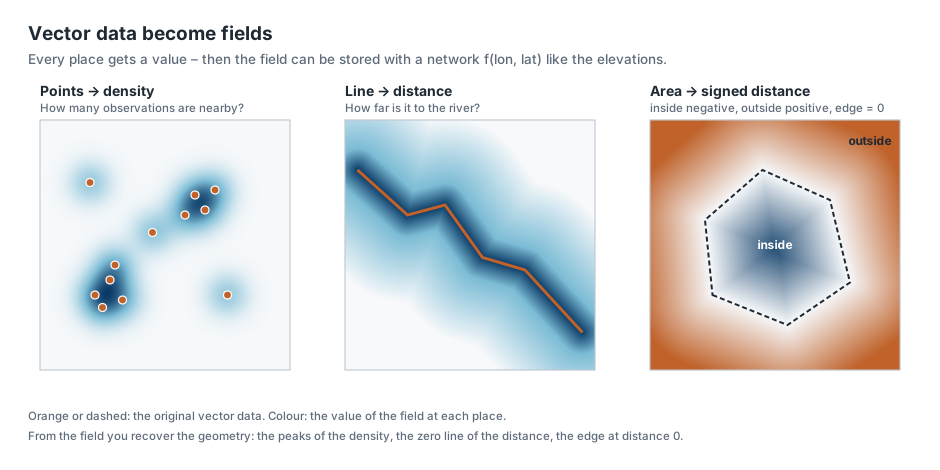
Three squares side by side. On the left twelve orange points, beneath them a blue area that is dark where many points lie close together. In the middle an orange line like a river, dark blue right at the line and lighter and lighter further out. On the right a dashed area, blue inside, orange outside, white at the edge.

Points become a density. For every place you ask: how many points lie nearby? Or, for sites where an animal species was found: how likely is it to encounter the species here? Cole and colleagues used this approach to learn the ranges of 47 000 animal and plant species with a single network, from millions of observations reported by volunteers [3]. Their network gets a coordinate and outputs a probability for each species – a field, as in this tutorial, only with 47 000 outputs instead of one.

If the points have measured values, such as temperatures at weather stations, the network learns the field between the stations directly. Unlike with the elevations, however, there is then no complete grid: the network has to generalise between a few points, and you need test data again as in ordinary training (chapter 2).

Lines become a distance. For every place you ask: how far is it to the nearest river, the nearest road, the coast? Right on the line the distance is zero; next to it, it grows evenly. Such a distance field is smooth and easy to learn.

Areas become a signed distance. For an area you take the distance to the edge and give it a sign: negative inside, positive outside. The edge itself is exactly the line where the field is zero. This representation is called a signed distance function. It became known for 3D shapes through DeepSDF by Park and colleagues [4]; Chu and Shahabi use the same idea for points, lines and areas in geodata [5]. Even simpler is a field that only says whether a place lies inside (1) or outside (0), such as "land or sea?" or "in which country does this point lie?".

Recovering the geometry. From the field you get the vector data back out: the peaks of the density, the zero line of the distance, the edge at zero. This can even be shown with the network of this tutorial. The coast is the line where the elevation is exactly 0 m:

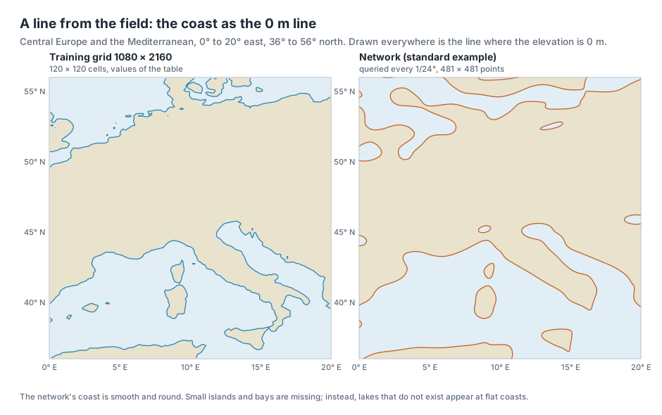
Two maps of Central Europe and the Mediterranean with the coast as the 0 m line. On the left from the training grid: fine, jagged coasts, Corsica, Sardinia, Sicily and small islands clearly visible. On the right from the network: smooth, round coasts, Corsica and Sardinia as soft blobs, small islands missing, and in some places inland there are lakes that do not exist.

By area, the standard example is on the correct side for 97 % of the Earth's surface – land where there is land, sea where there is sea. At the coasts themselves, in cells with elevations between −200 m and +200 m, it is only 80 %. Exactly where the line runs, the network is least certain.

The limits of this approach. Vector data are usually already very compact: a coastline is a list of coordinates, accurate to the centimetre. A field gives up this accuracy. It also knows nothing about rules that matter for vector data – that two neighbouring countries share exactly the same border, that a road is connected without gaps, or what a river is called. Whether a neural field saves storage for vector data is therefore an open question; it is useful above all when you need the data as a field anyway, such as "how far is every place from the nearest hospital?".

Approach 2: every object becomes a vector of numbers

The second approach does not want to store vector data but make it usable for machine learning. Many tasks need a geometry as input: is this footprint a house or a factory? Does this lake lie in that protected area? How many people live in this district?

But a network cannot process a list of coordinates of varying length. That is why an encoder translates every object into a vector of numbers of fixed length, for example 256 numbers. Similar objects should get similar numbers. These numbers are called an embedding.

Points: for a single place there are location encoders. They usually work with sine and cosine waves of many sizes – just like the Fourier features from chapter 5. Space2Vec by Mai and colleagues is an early example [6]; SatCLIP by Klemmer and colleagues learns the numbers for every place on Earth from satellite images [7]. Mai and colleagues give an overview of these methods [8].
Areas: Mai and colleagues describe a polygon encoder that captures the shape of an area via a Fourier transform. It is robust to the fact that the same area can be described in different ways, for example with a different starting point or additional vertices [9].
All three kinds: Poly2Vec by Siampou and colleagues treats points, lines and areas with the same method, also via a Fourier transform. With it, the network can recognise relations such as "touches", "lies north of" or "is 3 km away" between any objects [10]. The method by Chu and Shahabi from approach 1 also produces such vectors of numbers, from the distance field of each object [5].

Here the network is therefore not the file but a translator. The vector data stay as they are; the network additionally provides a representation that other networks can compute with.

The two approaches compared

	Approach 1: field	Approach 2: vector of numbers per object
Goal	store or query data as a function	make objects usable for machine learning
Input of the network	one coordinate	a whole object
Output	one value at this place	a vector of numbers of fixed length
Related to	this tutorial	the Fourier features from chapter 5
Examples	species ranges [3], distance fields [4, 5]	Space2Vec [6], SatCLIP [7], polygon encoder [9], Poly2Vec [10]

Common to both approaches is the basic idea of this series: instead of treating geodata as a table or a list, you describe them as a function – and let a network learn what this function looks like.

Ideas to explore further

In the Maps & Error tab, look at the error map at the coasts. Where would the network confuse land and sea?
Compare the coast from networks of different sizes, for example Fourier MLP, very small against Fourier MLP, large, in the Super-Resolution tab with a 2° window. From which size does the outline of Corsica match?
Think about which of your own geodata would suit a field well – and which badly. A helpful question: does the value have a meaning at every place, or only on individual objects?
If you know data from OpenStreetMap: for a city, compute the distance of every place to the nearest stop as a grid. That is a field as in approach 1 – and could be trained with the app just like the elevations if you add it as a data source.